
FS-1046 | January 2017
Precision Soil Sampling Helps Farmers Target Nutrient Application
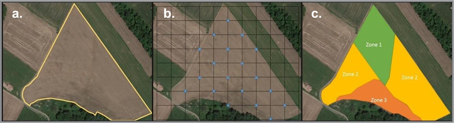
Precision agriculture allows modern producers to manage within fields rather than managing the whole field.¹,² By integrating global positioning systems (GPS), variable rate (VR) application equipment, and geographic information systems (GIS), farmers are allowed increased efficiency. However, prior to using VR equipment, accurate maps of yield-limiting factors must be created.³,⁴,⁵ Nutrients in any field vary due to topography, soil properties and past management (manure application patterns, crop history, etc.). To account for this variability, farmers will need more than one soil sample in each field (Figure 1a). A more intensive sampling scheme must be performed, through either grid or zone sampling. Looking to the future, on-the-go sensors, whether attached to tractors or unmanned aerial vehicles, may also increase accuracy and decrease the cost of soil sampling.
Grid Sampling is a Well-established Method that is Simple to Understand
To manage a field by the grid method, a layer of equally spaced, intersecting lines is lain over a map or photograph of the field (Figure 1b). Compared to the whole-field method (Figure 1a), many more samples will be taken. The easiest way to create a grid is through GIS software, which can be expensive, although there may be free or cheaper alternatives (e.g. QGIS). A farmer may also create a grid on transparent paper, which may be overlain on a map of the field.⁴
Grid size is important, since smaller-sized grids would mean more samples to analyze. Consider a 40-acre field where a farmer overlays a map of equally sized squares (e.g. 2-acre grid). The farmer would collect 20 samples for the entire field (40 acres divided by the 2-acre grid). If each soil sample costs $10 to analyze, the total cost would be $200 for the 40 acres. This is expensive, yet it is important to remember that these maps are meant to last for several years, and not repeated annually.
The labor in a 40-acre field should also be considered, since those 20 samples should be a composite sample of at least 5 cores. That makes at least 100 cores to be collected on 40 acres, a significant amount of work.
Other costs of grid sampling include the software to create the grids and GPS equipment to find each sample location. To be of value, grid maps should result in lower seed, fertilizer and lime application use and costs based on the additional information garnered from grid sample analysis. Sampling costs should not exceed the returns from higher yields or lower input use.⁶,⁷ It may make more sense to pay a trained consultant to collect these samples and create the grids.
Studies of Grid Sampling Focused on the Ideal Size
Larger grid sizes require fewer samples, but they are also less accurate. Some studies have found that grids larger than one third and up to 2 acres may not capture soil variability.⁸,⁹ The University of Nebraska recommends a maximum of one sample per acre, although one per 2.5 acres will work if there is less variability.³,¹⁰
The optimal grid size depends on how soils vary across the farm. For each field, consulting soil and yield maps may provide an initial idea of variability. Drainage, topography and previous manure application should also be considered. The grid spacing should also not overlap with established field patterns, including old field boundaries or drainage ditches.⁴ Areas closest to a barn may also have received more manure applications.³
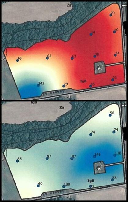
In Figure 2, grid sampling uncovered variable phosphorous (P) and potassium (K) levels in the soil, either due to topographic differences or previous nutrient application. Studies of grid sampling indicate smaller grid sizes of one acre enable better predictions of soil P and K levels.³,⁸ To map organic matter and clay, one sample per 5 acres has been adequate (Table 1).⁸ In fields where known soil properties are fairly similar spatially, grid sampling is probably not economically suitable.⁶ However, this may not be apparent until after the grid sampling is performed.
For further guidance on creating grids, please read the guide from the University of Nebraska: Soil Sampling for Precision Agriculture (EC154).³
| Recommended Grid Sizes | |
| 1 to 2.5 acres | P, K, pH |
| 5 acres | Organic matter, Texture |
| Lifetime Map Usefulness | |
| 5 years | P, K |
| 10 years | pH |
| 10-20 years | Organic matter, Cation exchange capacity, Texture |
| *Indicates how long an initial map may be used, soil samples may still be used to check the map and make recommendations | |
When Performed at the Correct Scale, Grid Sampling Maps Remain Accurate for Years
It is not necessary to create new soil sampling grids yearly. Maps for slowly changing landscape properties, such as organic matter and cation exchange capacity, can last 10 to 20 years (Table 1). Maps of relative nutrient content and pH will have shorter, but still significant life spans of 5 and 10 years, respectively.³ These are suggested lifetime uses of a map, but do not suggest that annual soil sampling should not be performed to check map accuracy.
In Illinois, 40 years of grid sampling revealed that initial nutrient patterns remained the same due to intrinsic soil properties.¹¹ This indicates that while the nutrient content and pH of soils may change, the relative differences across a field may not.
In Maryland, it is important to remember that soil samples must be taken every three years. However, previous grid sampling could allow for limited sampling in known high- and low-yielding areas of the field. This also leads another precision sampling method: management zones.
Management Zones are Less Labor Intensive, but Require More Brain Power
Grid sampling has been described as too expensive to be cost effective for farmers.⁷ To alleviate the labor and cost of grid sampling, management zones were developed (Figure 1c). Management zones are designed to group similar-yielding sections of a field. Instead of intensive grid sampling, soils can be grouped as a consolidated sample within each zone (high, average, and low yield).
Conveniently, these zones don’t have to be restricted to one field. If similar yield-limiting factors are observed across a farm (soil type, organic matter, available water), samples could be combined from those fields into one zone. Management zones can lower the amount of samples needed, but the result may be less sensitive in detecting small field variations.⁵
To Create Management Zones, Several Layers of Data may be Necessary
A management zone is created by combining several layers of data that correlate to yield potential. For example, combining topography, soil survey maps and yields can uncover regions that have similar yield potential. Table 2 lists several types of maps.
Soil survey maps created by the U.S. Department of Agriculture’s Natural Resource Conservation Service are too coarse (don’t capture variability) for VR application.⁷ Soil surveys can be useful when combined with known field characteristics that affect yield. These characteristics include soil texture; pH; nutrient content; organic matter; and available water.¹⁰,¹²
| Map Type | Soil Characteristics |
|---|---|
| Grid | Nutrients, pH, organic matter |
| Soil Survey Topography Aerial photos |
Texture Predict runoff/leaching Soil color, normalized difference vegetation index (NDVI) |
| Yield Maps EC Maps pH Maps |
Actual yearly harvest Texture, water holding Soil pH |
Creating and obtaining accurate maps of soil properties is more difficult. An initial grid sampling is one way to determine properties like texture, pH and organic matter, that don’t change quickly (Table 2).¹ Topographic maps may be useful, but are often already correlated to the original soil map.
Remote sensing technologies can provide accurate and useful maps, including satellite and aerial photos using visual and infrared light. Soil color is one characteristic of aerial photos which can be directly related to organic matter and texture.¹³,¹⁴ Soil color can also be complicated by tillage practices.
After crops are planted, aerial photos can be used to calculate the normalized difference vegetation index (NDVI), which measures how green, or healthy, a plant is.¹³
Field equipment may also collect data, such as yield maps, soil electrical conductivity (EC) and pH. Yield maps are a well-established precision agriculture technology, collected by equipment (e.g. combines) and marked using GPS. Maps of EC can also be created with specialized equipment, which can correlate conductivity to water content and soil texture.¹⁵,¹⁶
The More Correlated to Actual Yield, the More Useful the Map
Soil color has been a better predictor of management zones than actual yield maps in the western United States.⁷,¹⁴ This is probably related to soil organic matter content as well as texture, which may control N availability and water holding.
Early in the season, NDVI has also provided a strong aerial agreement with grain yield. However, it does not provide much more information when combined with soil color-based zones.¹³
Maps of EC are helpful for differentiating soil texture, moisture and carbonate content but doesn’t correlate well with yield.¹⁴ In fields with large variability in texture (e.g coastal or alluvial soils), EC may provide better correlation with yields.¹⁵ Conductivity, when combined with yield, soil color or topography, provides beneficial information for creating management zones. Farmer knowledge, soil tillage, crop rotations or old field boundaries are also useful for creating management zones.
Harvest yield maps may initially appear to be the most useful layer to predict future yields, but weather, disease and management reduce their accuracy. At least three years of yield data should be averaged to cover seasonal variability and producer error.⁹
Averaging yield map data must be done carefully. The highest-yielding portion of a field may be 200 bushels one year, but reduced to 160 bushels the next year due to drought. To counter this effect, data can be normalized. One way would be to divide by the greatest yield each year. That way, the highest yielding portions will have a value of “1” for each year (200/200 or 160/160), and all other yields will be less than 1. These maps will provide a better “average” yield potential.
Another method of normalizing yield is to use GIS software to calculate the relative yield for each crop (Table 3). For example, the average yield for each crop would have a relative yield of 100. Locations in the field where the yield monitor registered above the average would have a relative yield above 100 and points registering below the average would have a relative yield below 100. This method could be used across several crop types in the same field.
| Year | Crop | Highest Yield | Normalized Yield | Average Yield | Normalized Yield | Lowest Yield | Normalized Yield |
|---|---|---|---|---|---|---|---|
| 2014 | Corn | 187 | 115 | 163 | 100 | 135 | 83 |
| 2015 | Wheat | 57 | 118 | 57 | 100 | 52 | 91 |
| DC Soybeans | 47 | 115 | 41 | 100 | 37 | 90 | |
| 2016 | Soybeans | 58 | 109 | 53 | 100 | 47 | 89 |
| Average | 114 | 100 | 88 | ||||
| Zone | 1 | 2 | 3 | ||||
The Number of Management Zones is Another Important Choice
Some studies of management zones have classified three zones as low-, average- and high-yielding.¹⁰,¹⁴ Significant differences were often only observed between low- and high-yielding zones (i.e. average was similar to both high and low zones in crop yield).⁷,¹⁴ Even when there is not much difference between zones, the average zone provides a transition between low and high zones, and improves the usefulness of the map. Although zones have sharp boundaries, soil properties actually transition. The edge of Zone 1, for example, could fall into the adjacent zone, while the center is often classified for the correct yield (Figure 1c). It is important that each zone have very similar yield potential within, but be as different as possible from other zones.5 In fields with drastically changing soil types, this may be easier to achieve (e.g. Coastal soils with varying clay content).¹⁵
Fields with a lot of soil variability may have the potential for more than three zones. However, if the yield-limiting factors in a field do not vary a lot, more than three zones may not be worth the effort. For example, it may be easy to separate a sandy soil from one higher in clay in one field, but two soils with slightly different clay content may not be worth the effort.
Another consideration is the width of equipment.¹⁴ As fields are split into smaller management zones, they must still be wider than the equipment used for seed, fertilizer and lime application. It is probably a good idea to start with three zones, and then determine if more are needed. This may best be performed by personal knowledge of a field. If zone management has missed obvious differences in the field, adjustments in classification or zone number may increase the accuracy.
Most of the Savings from Management Zones Comes From Lower N Application
Precision management has not necessarily increased yields compared to traditional soil sampling.⁵ Instead, cost savings have been observed due to lower nutrient application in low-yielding zones.⁶ In other words, low-yielding regions of a field, possibly due to poor soil productivity, may be receiving excess nutrients that do not contribute to yield. Lower N applications to poor soils have reduced production costs.⁶
Precision soil sampling is more profitable for larger farm sizes, when sampling cost is reduced and when a farmer can spread the use of VR equipment over several uses (e.g. nutrient application and pesticide application).⁶, ¹⁷ In some cases, custom services may be more appropriate than purchasing on-farm equipment.
Does Nutrient Management in Maryland Affect my Variable Rate Application?
In Maryland, nutrient application for field crops, vegetable, or fruit production may require a nutrient management plan (NMP). This plan will specify the amount of nutrients that can be applied based on factors such as crop and soil type and risk to water quality.
Traditionally an NMP has been written for a whole field, where one sample may represent 40 acres. For precision agriculture, the increased number of samples (40 acres = 20 samples) can make an NMP much more complicated. To make use of a grid sampling scheme, each sample point could make up a single recommendation. For management zones, an NMP could potentially be much shorter, since zones could be combined across the farm for regions with similar yield potential.
However accurate they are, grid or zone maps cannot exceed the recommended rate. If precision sampling uncovers large differences in crop needs across a field, the effort to incorporate into a NMP may be worth the effort. However, if the variability across a field is not that great, a whole field sample may do.
The Choice in Sampling Method Will Rely on the Method and Cost Involved
Whether a farmer chooses the classic whole-field or grid/zone methods, the costs and benefits may not be easily determined. Two immediate questions to ask are 1) do yields vary significantly across these fields and 2) is precision agriculture equipment economically available to this operation? If the answer is yes to both of these questions, it is feasible to examine whether grid or zone sampling could reduce production costs.
Technology will continue to improve while costs will fall, allowing reexamination in the future. Long term data collection and known soil properties could be combined with in-field sensors (unmanned aerial vehicles, greenseeker) to improve yields during the season.
References
- Grisso, B, M.M. Alley, P. McClellan, D. Brann, and S. Donohue. 2009. Precision Farming: A Comprehensive Approach. Virginia Cooperative Extension. Publication 442-500.
- Davis, G, W. Casady, R. Massey. Precision Agriculture: An Introduction. University of Missouri Extension System. WQ-450.
- Ferguson, R.B. and G.W. Hergert. 2009. Soil Sampling for Precision Agriculture. University of Nebraska Extension. EC154.
- Wollenhaupt, N.C. and R.P. Wolkowski. 1994. “Grid soil sampling,” Better Crops. 78(4): 6-9.
- Mallarino, A. and D. Wittry. 2001. Management zones soil sampling: A better alternative to grid and soil type sampling? 13th Annual Integrated Crop Management Conference. Ames, IA.
- Koch, B., R. Khosla, W.M. Frasier, D.G. Westfall, and D. Inman. 2004. "Economic feasibility of variability-rate nitrogen application utilizing site-specific management zones". Agron. J. 96:1572-1580.
- Hornung, A., R. Khosla, R. Reich, D. Inman, and D.G. Westfall. 2006. “Comparison of site-specific management zones: soil color based and yield based,” Agron. J. 98:407-415.
- Nanni, M.R. et al. 2011. “Optimum size in grid soil sampling for variable rate application in site-specific management,” Sci. Agric. 68(3): 386-392.
- Mallarino, A.P. and D.J. Wittry. 2004. “Efficacy of grid and zone soil sampling approaches for site-specific assessment of phosphorus, potassium, pH, and organic matter,” Precision Agric. 5:131-144.
- Doerge, T. 1999. Management Zone Concepts. SSMG-2. Potash and Phosphate Institute. Retrieved from http://www.ipni.net/ on January 15, 2016.
- Franzen, D.W. 2007. Lessons Learned from 40 Years of Grid Sampling in Illinois. 2007. Indiana CCA Conference Proceedings.
- Mzuku, M., R. Khosla, and R. Reich. 2015. “Bare soil reflectance to characterize variability in soil properties,” Comm. in Soil Sci. Plant Anal. 46(13): 1668-1676.
- Inman, D, R. Khosla, R. Reich, and D.G. Westfall. 2008. “Normalized difference vegetation index and soil-color based management zones in irrigated maize,” Agron. J. 100(1): 60-66.
- Khosla, R., D. Inman, D.G. Westfall, R.M. Reich, M. Frasier, M. Mzuku, B. Koch and A. Hornung. 2008. “A synthesis of multi-disciplinary research in precision agriculture,” Precision Agric. 9:85-100.
- Anderson-Cook, C.M., M.M Alley, J.K.F. Roygard, R. Khosla, R.B. Noble, and J.A. Doolittle. 2002. “Differentiating soil types using electromagnetic conductivity and yield maps,” Soil Sci. Soc. Am. J. 66:1562-1570.
- Shaner, D.L., R. Khosla, M.K. Brodahl, G.W. Buchleiter, and H.J. Farahani. 2008. “How well does zone sampling based on soil electrical conductivity maps represent soil variability?” Agron. J. 100(5): 1472-1480.
- Griffin, T., D. Lambert and J. Lowenberg-DeBoer. 2005. Economics of Lightbar and Auto-guidance GPS Navigation Technologies. 5th European Conference on Precision Agriculture1580.
JARROD O. MILLER
CRAIG W. YOHN
cyohn@umd.edu
This publication, Precision Soil Sampling Helps Farmers Target Nutrient Application (FS-1046), is a part of a collection produced by the University of Maryland Extension within the College of Agriculture and Natural Resources.
The information presented has met UME peer review standards, including internal and external technical review. For help accessing this or any UME publication contact: itaccessibility@umd.edu
For more information on this and other topics, visit the University of Maryland Extension website at extension.umd.edu
University programs, activities, and facilities are available to all without regard to race, color, sex, gender identity or expression, sexual orientation, marital status, age, national origin, political affiliation, physical or mental disability, religion, protected veteran status, genetic information, personal appearance, or any other legally protected class